Recently, I found myself needing to implement this functionality. While someone with a background in mathematics from a computer science university could probably figure this out on their own, after searching online, I couldn’t find any existing solutions, so I’ll document the method here.
Inverse Transform Method
For any probability distribution, if you can determine its cumulative distribution function ($F(x)$ = the probability that a randomly generated value is less than or equal to $x$) and its inverse function, you can generate a random variable following that distribution. Simply pass a uniform random variable $U$ uniformly distributed in $[0,1)$ to the inverse function.
$$ X := F^{-1}(U) $$
The person who first conceived of this method must have been a true genius.
Inverse Gaussian Distribution
With this approach, we can now generate random variables for any probability distribution whose cumulative distribution function’s inverse is known. We can use this technique to create the random wait times we need.
When discussing waiting times, queueing theory comes to mind. Among the distributions commonly encountered in queueing theory are Poisson distributions, which have both mean and variance determined by a single parameter.
They’re convenient for theoretical analysis when calculations are straightforward, but become problematic when you want to freely adjust the variance or mean.
Browsing through various probability distributions on Wikipedia, I came across the inverse Gaussian distribution.
Inverse Gaussian distribution - Wikipedia
This distribution has two parameters: $\mu$ and $\lambda$, with the expectation value (mean) equal to $\mu$ and the variance equal to $\mu^3/\lambda$. This means that as long as the mean $\mu$ is not zero, you can freely set both the mean and variance. The cumulative distribution function for this distribution is as follows:
$$ F(x) = \Phi\left(\sqrt{\frac{\lambda}{x}}\left(\frac{x}{\mu}-1\right)\right) + \rm{exp}\left(\frac{2\lambda}{\mu}\right)\Phi\left(-\sqrt{\frac{\lambda}{x}}\left(\frac{x}{\mu}+1\right)\right) $$
$$ \Phi(x) = \frac{1}{2}\left(1 + \rm{erf}\left(\frac{x}{\sqrt{2}}\right)\right) $$
Here, $\rm{erf}(x)$ is the Gaussian error function, which is typically available in mathematical libraries.
In Go, it’s included in the standard library. Just to clarify, $\rm{exp}(x)=e^x$.While solving for the inverse of this complex cumulative distribution function seems challenging, by definition the cumulative distribution function is monotonically increasing, so you could approximate it using methods like binary search or Newton’s method.
Implementation
With that in mind, let’s implement it. First, the cumulative distribution function for the inverse Gaussian distribution: inverseGaussianDistributionCDF.
func standardNormalDistributionCDF(x float64) float64 {
	e := math.Erf(x / math.Sqrt(2))
	return (1 + e) / 2
}

func inverseGaussianDistributionCDF(x float64, mu float64, lambda float64) float64 {
	a := math.Sqrt(lambda/x) * ((x / mu) - 1)
	b := math.Exp(2 * lambda / mu)
	c := -math.Sqrt(lambda/x) * ((x / mu) + 1)
	return standardNormalDistributionCDF(a) + b*standardNormalDistributionCDF(c)
}
Next, we’ll implement the inverse of the cumulative distribution function using this implementation. Since pure binary search would be too slow, I tried using Newton’s method, but I’ve included conditional checks to suppress occasional NaN values, so it’s probably buggy.
Here’s the code:
func (ig *InverseGaussianDistribution) InverseCDF(y float64) float64 {
	if y <= 0 || 1 <= y {
		return math.NaN()
	}
	// Newton's method implementation
	x := 1.0
	for i := 0; i < 50; i++ {
		a := y - ig.CDF(x)
		b := -ig.PDF(x)
		if math.Abs(a/b) < 0.1 || math.IsInf(a/b, 0) || math.IsNaN(a/b) {
			break
		}
		x = x - a/b
	}

	// Binary search implementation
	less := math.Max(0, x-0.25)
	more := math.Max(0, x-0.25) + 0.5
	for i := 0; i < 50; i++ {
		m := less + (more-less)/2
		if ig.CDF(m) < y {
			less = m
		} else {
			more = m
		}
	}
	return less
}
Finally, by passing a uniform random number to the inverse function, we’re done.
func (ig *InverseGaussianDistribution) Float64() float64 {
	return ig.InverseCDF(ig.rng.Float64())
}
The complete code is available here. It’s set up as a usable library.
kotet/igaussian: Go library providing Inverse Gaussian distributions
Results
Let’s generate approximately 10,000 samples with $\mu=1$ and $\lambda=3$ and plot a histogram.
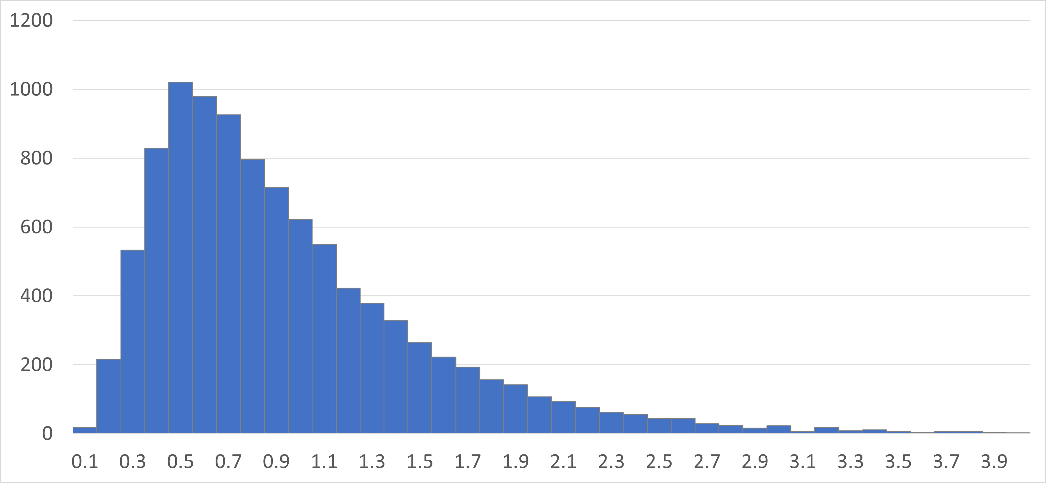
At this point, I finally realized that in practical applications, it’s not the expected value that’s crucial—it’s the mode that matters. While the expected value should be $\mu$=1, the mode appears around 0.5. We should look for a distribution where controlling the mode is more straightforward. Though I intended to continue searching for such a distribution, I ran out of energy, so I’ll conclude the discussion here.